4  TIMSCONVERT workflow comparison

4.1 Introduction

In this part, we compare TIMSImaging workflow with existing method that ignores ion mobility on the same mosue kidney peptide dataset. TIMSCONVERT is an open-source tool to convert general Bruker raw data into open formats, users could install from https://github.com/gtluu/timsconvert. Specifically, it outputs imzML for MALDI-TIMS-MS imaging data, either with ion mobility or not. However, it does NOT do any pre-processing.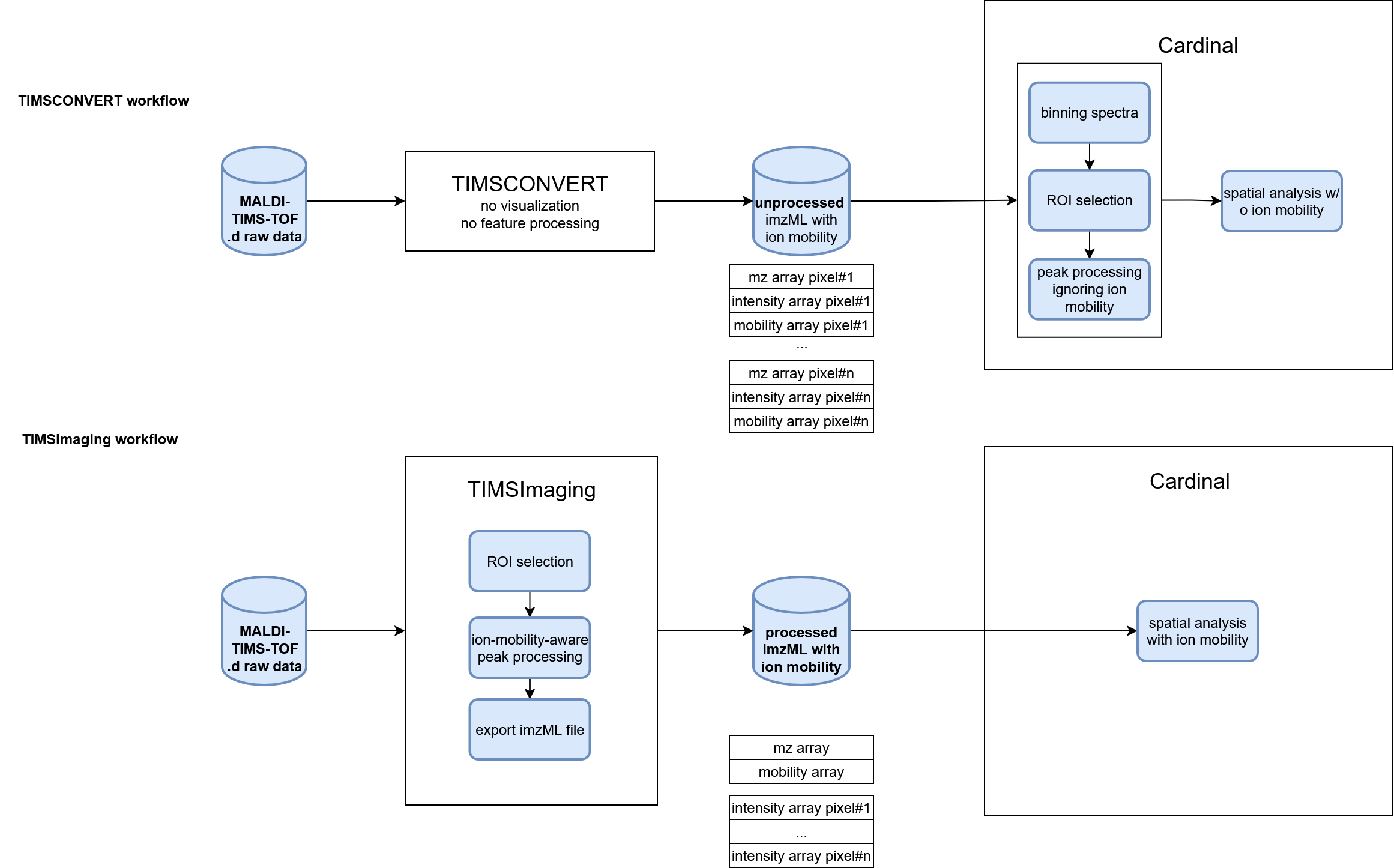

4.2 Convert raw data using TIMSCONVERT

First we run the shell script below to convert the raw dataset into unprocessed imzML using TIMSCONVERT. Note that unprocessed imzML of TIMS-on dataset is usually huge, we recommmend to do the conversion on HPC.

#!/bin/bash
#SBATCH --nodes=1
#SBATCH --time=4:00:00
#SBATCH --job-name=Casestudy_timsconvert
#SBATCH --mem=80G
#SBATCH --partition=short
#SBATCH -o output_%j.txt                    # Standard output file
#SBATCH -e error_%j.txt                     # Standard error file
#SBATCH --mail-user=zhu.yiny@northeastern.edu  # Email
#SBATCH --mail-type=ALL                     # Type of email notifications
eval "$(conda shell.bash hook)"
conda activate timsconvert
cd /work/VitekLab/Data/MS/Melanie_manuscript/
timsconvert --input Kidney_MS1_ITO6.d --outdir mouse_kidney_timsconvert_output --compression none --mode centroid --verbose
conda deactivate

4.3 Process data from TIMSCONVERT

Load the imzML data from TIMSCONVERT:

msa <- readMSIData("D:\\dataset\\Melanie_case_study\\Kidney_MS1_ITO6.imzML")
msa

MSImagingArrays with 38267 spectra 
spectraData(2): intensity, mz
pixelData(3): x, y, run
coord(2): x = 204...753, y = 99...442
runNames(1): Kidney_MS1_ITO6
experimentData(5): spectrumType, spectrumRepresentation, lineScanSequence, scanType, lineScanDirection
centroided: TRUE 
continuous: FALSE 

TIMSCONVERT keeped the ion mobility array in the imzML data, however the peak processing functions in Cardinal cannot take advantage of it. When loaded into MSImageExperiment, the ion mobility array is discarded, and data points with the same m/z but different ion mobilities can no longer be distinguished, but they are still separate entries. Here we bin the spectra to project isobaric data points together, then do processing without ion mobility in Cardinal.

mse_binned <- bin(msa, resolution=20, units="ppm")
mse<-summarizePixels(mse_binned)

To reduce the computation, we only process the kidney tissue region in following steps.

kidney <- subsetPixels(mse, x<500)
image(kidney, 'tic')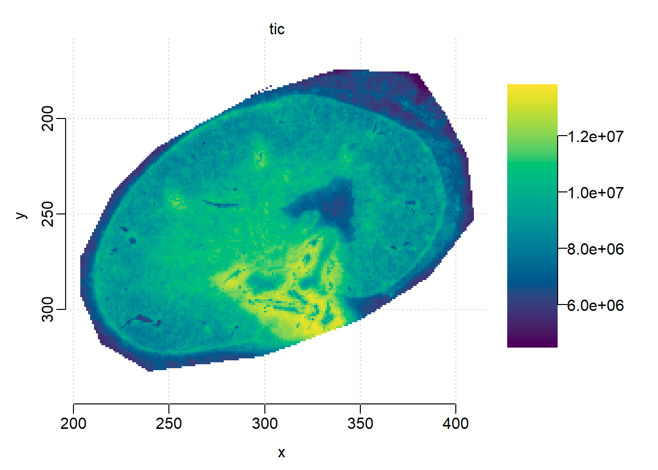

Plot one spectrum, though a single spectrum is centroided on m/z dimension by the instrument, it looks more similar with a profile spectrum after projection.

plot(kidney, i=1234)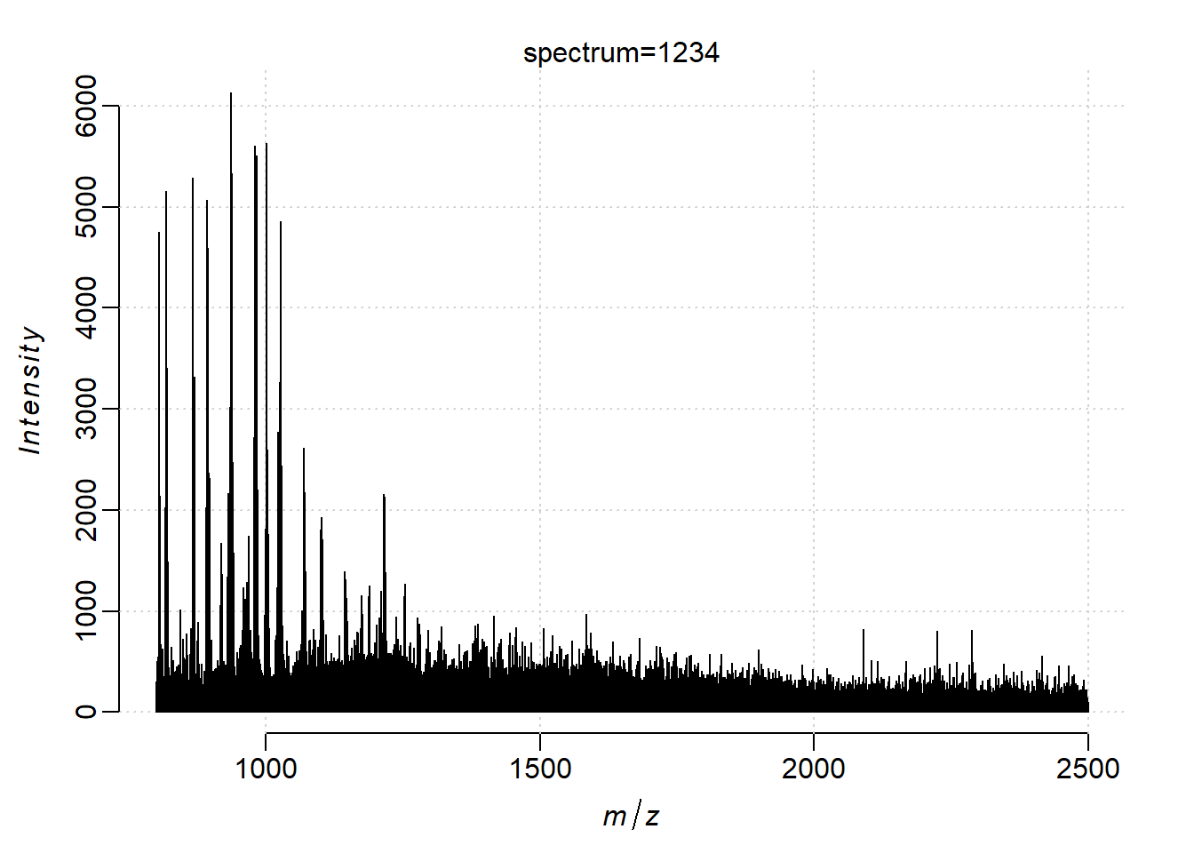

Treat the data as profile spectra and process it to reduce the number of features.

kidney <- subsetPixels(mse_binned, x<500)
centroided(kidney)<-FALSE
set.seed(1, kind="L'Ecuyer-CMRG")
#kidney <- normalize(kidney, method='rms')
peaks <- peakProcess(kidney, SNR=3, tolerance=200, units="ppm")

4.4 Comparing ion images with/without ion mobility

Then we load the processed data from TIMSImaging, which is already peak-picked.

peaks_timsimaging <- readMSIData("D:\\dataset\\Melanie_case_study\\mouse_kidney.imzML")
peaks_timsimaging

MSImagingExperiment with 3110 features and 22978 spectra 
spectraData(1): intensity
featureData(1): mz
pixelData(3): x, y, run
coord(2): x = 204...409, y = 175...332
runNames(1): mouse_kidney
experimentData(5): spectrumType, spectrumRepresentation, lineScanSequence, scanType, lineScanDirection
mass range:  800.2957 to 1760.7449 
centroided: TRUE 

Normalize on peak-picked data for fair comparison:

peaks_norm = process(normalize(peaks, method='tic'))
peaks_timsimaging <- process(normalize(peaks_timsimaging, method='tic'))

Plot ion images from processsing with/without ion mobility in the same color scale.

m <- 1198.7
image(peaks_timsimaging, i = findInterval(m, mz(peaks_timsimaging))+1, zlim=c(0, 5))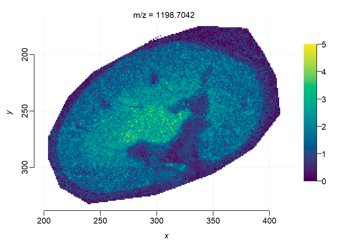

image(peaks_norm, mz = m, zlim=c(0, 5))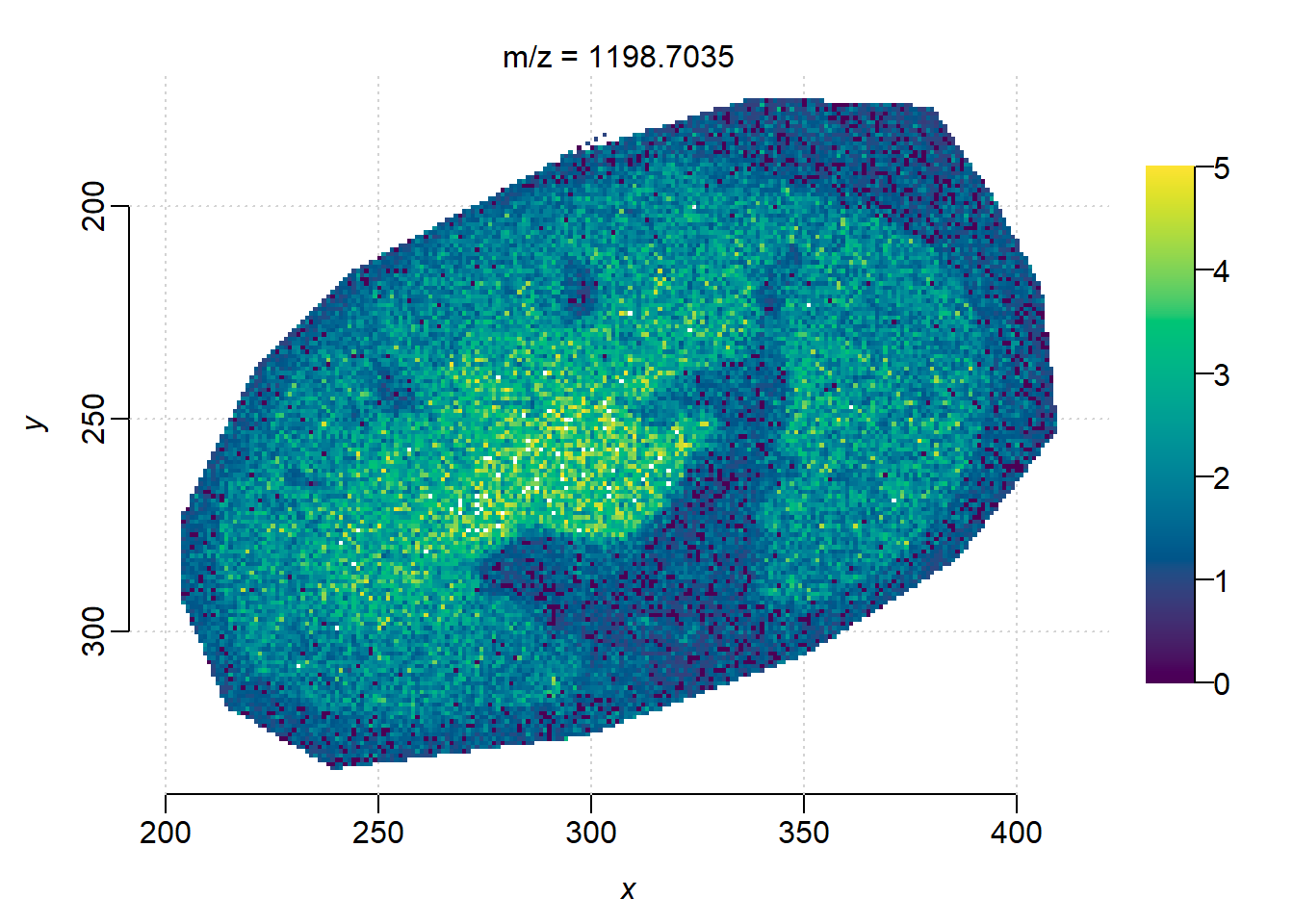

The ion images from TIMSCONVERT and processed in Cardinal looks noiser, as well as less contrast between the background and kidney edge.

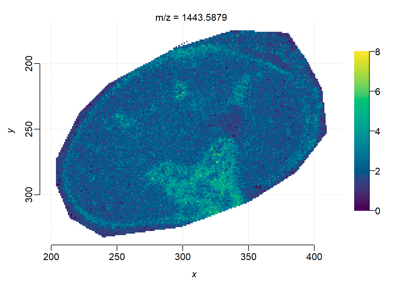
m <- 1443.59
image(peaks_timsimaging, i = findInterval(m, mz(peaks_timsimaging))+1, zlim=c(0, 8))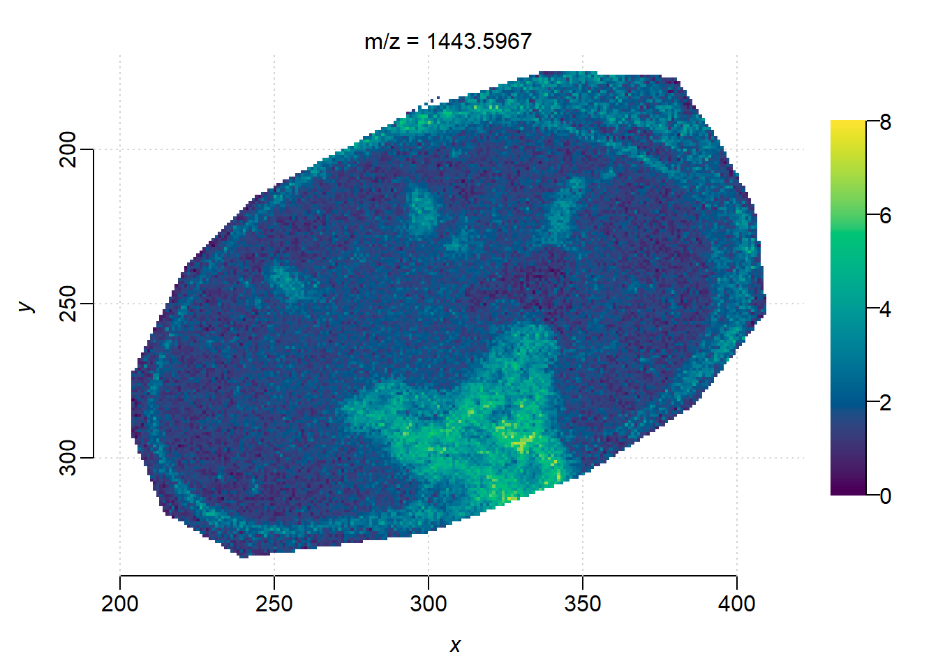

image(peaks_norm, mz = m, zlim=c(0, 8))